Project Overview
The goal of this project is to analyze the Fannie Mae Single-Family Loan Data.
What question am I trying to answer?
- The purpose is to build a model that can predict if an acquired loan will default or not.
Where to obtain the data?
All of the data came from Fannie Mae’s data housing website, and is broken up by quarters from 2000 through 2020.
The data used?
This project only used the following years: 2016, 2017, 2018, and 2019.
Original Data
Fannie Mae has all of its data in CSV format, and the total size is 370Gb. Each quarter starting has about 104 million rows, so altogether that would have required a massive amount of computing power.
The features for this data add up to108 columns; however, most of them were added in 2017 and would not start reporting data until June 2020, so I decided not to use those rows for this project.
Pre-Processing the data
Foreclosurehas 99.95% missing data andCo-Borrower Credit Score at Originationhas 52.79% missing.
Data Manipulation
Created a new column called Minimum Credit Score by taking the following columns:
-
Borrow Credit Score at Origination
-
Co-Borrower Credit Score at Origination
Guidelines provided by Fannie Mae state:
- If both columns have data use the lowest score
- If only one column has data use that score
- If neither columns have data take the mean of both and use the lowest score
Feature On Assistance Plan was mapped using the following code snippet:
# F T R to be on plan
def check_plan(x):
    if x in ['F', 'T', 'R']:
        return 1
    return 0
Dropped the following columns after creating new ones Borrower Credit Score at Origination, Co-Borrower Credit Score at Origination, Borrower Assistance Plan
Set new conditions to fill in the null values of Foreclosed using the following methods:
# df['Current Loan Delinquency Status'] >= 4 and not on df['On Assistance Plan'], foreclosed = 1 (True)
# create a list of our conditions
conditions = [
    (df['Current Loan Delinquency Status'] >= 4) &
    (df['On Assistance Plan'] == 0),
    (df['Foreclosure Date'].notnull())
    ]
# create a list of the values we want to assign for each condition
values = [1,1]
# create a new column and use np.select to assign values to it using our lists as arguments
df['Foreclosed'] = np.select(conditions, values)
with the final output of
0    8260646
1      22843
Name: Foreclosed, dtype: int64
The feature columns that were dates needed to be strings so we could format them correctly:
df[['Monthly Reporting Period',
        'Origination Date',
        'Maturity Date']]  = df[['Monthly Reporting Period',
                                    'Origination Date',
                                    'Maturity Date']].astype('str')
After imputation from float to string, the string retained its ‘.’, so to resolve this, a new column was created:
Origination Date
# new data frame with split value columns
df['Origination Date'] = df['Origination Date'].str.split(".", n = 1, expand = True)

df['Origination Date'] = pd.to_datetime(df['Origination Date'],format='%m%Y')
Maturity Date
# new data frame with split value columns
df['Maturity Date'] = df['Maturity Date'].str.split(".", n = 1, expand = True)

df['Maturity Date'] = pd.to_datetime(df['Maturity Date'], format='%m%Y')
Monthly Reporting Period
df['Monthly Reporting Period'] = pd.to_datetime(df['Monthly Reporting Period'],format='%m%Y')
Our final shape of the data (8,278,657, 19)
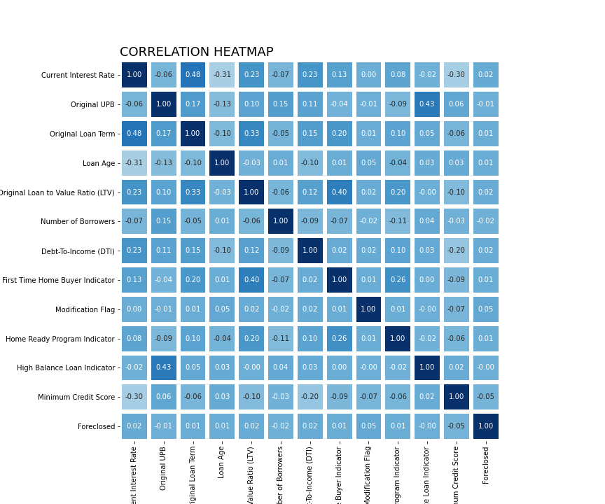
Exploratory Data Analysis
Reviewing the heatmap, we can see the relationship between all of the features and determine if there will be any collinearity; however, since we are conducting a prediction classification, multi-collinearity will not affect our outcome
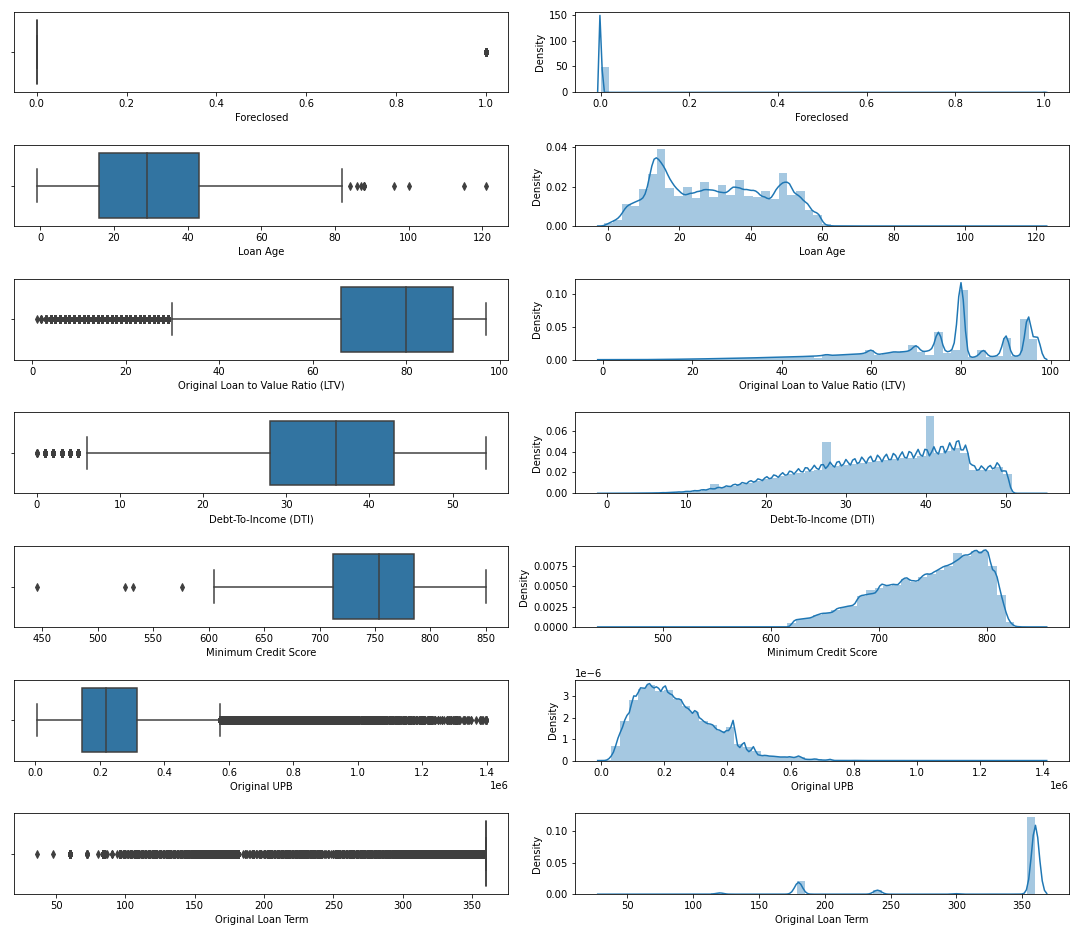
This image contains boxplots and distplots of a few features. We can see that some features include outliers, and we have right-skewed and left-skewed distribution.
Our target feature Foreclosed was heavily imbalanced:
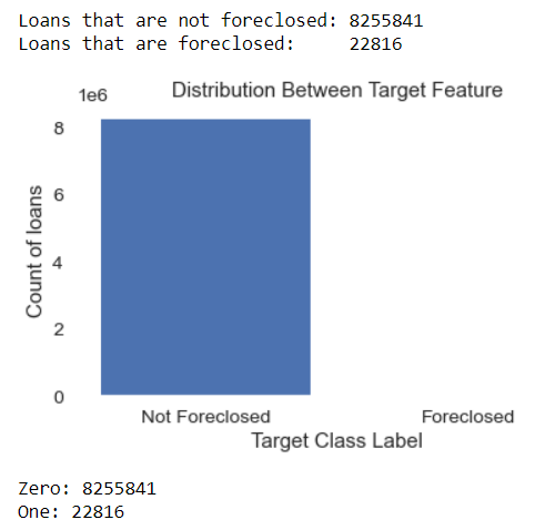
Imbalanced Data Modeling
Machine learning algorithms work better when the number of samples in each class are the same.
Here are some ways to overcome the challenge of imbalanced:
Can we collect more data?
- At this point this is all the data provided
- We can wait until there is more data from Fannie Mae
Change the performance metric.
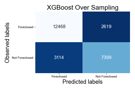
- Confusion Matrix: A breakdown of predictions into a table showing correct predictions and the types of incorrect predictions made.
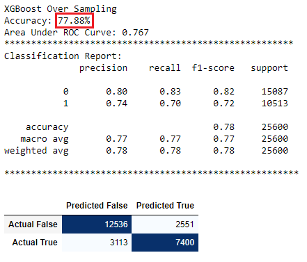
- Precision: A measure of a classifier’s exactness.
- Recall: A measure of a classifiers completeness
- F1 Score (or F-score): A weighted average of Precision and Recall.
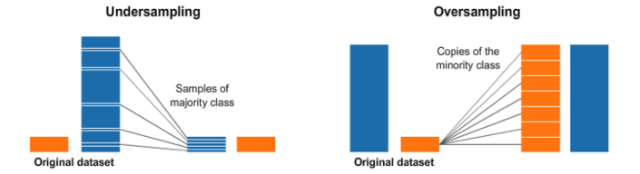
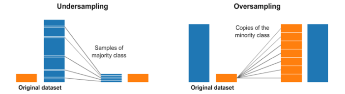
We can try resampling the dataset
- Add copies from the under-represented class called over-sampling, or
- Delete instances from the over-represented class, called under-sampling
- Or we could do both
I decided to generate synthetic samples
Here is a link to the most popular algorithm called Synthetic Minority Oversampling Technique known as SMOTE .
The module works by generating new instances from existing minority cases that you supply as input. This implementation of SMOTE does not change the number of majority cases.
Here is an example of what SMOTE is doing:
Models
- Logistic Regression
- Decision Tree
- Random Forest
- XGBoost
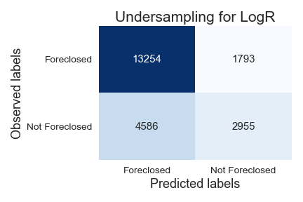
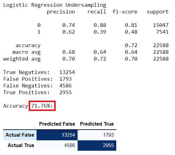
Logistic Regression
To create a baseline for all of our modelings, I ran a logistic regression algorithm. It is the simplest of all machine learning algorithms.
Logistic Regression Under Sampled
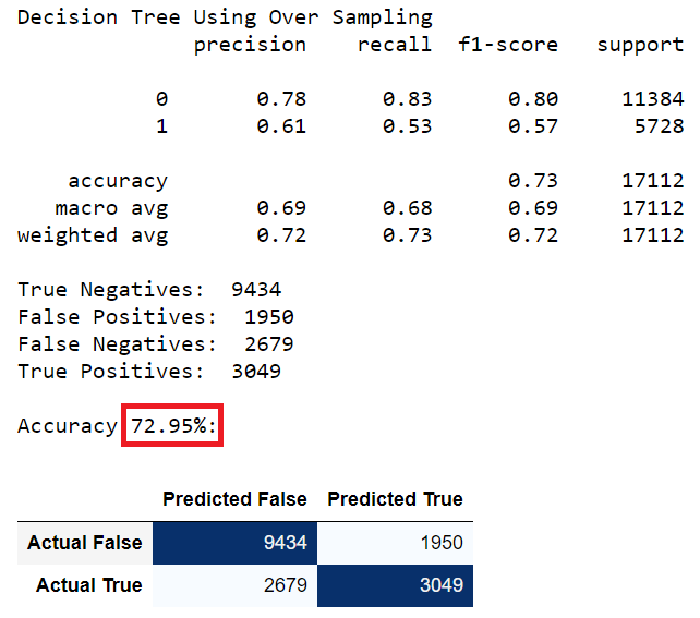
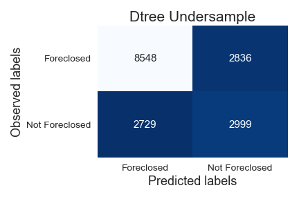
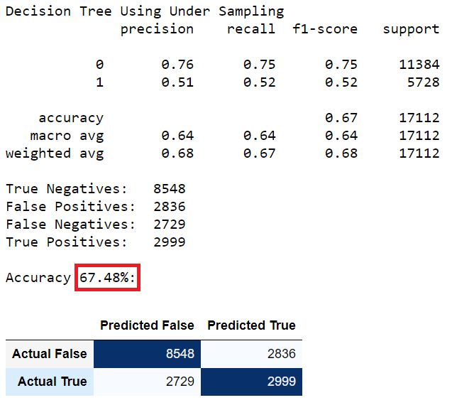
Decision Tree
Decision Tree using Over Sampling Data

Random Forest
Random Forest using Under Sampling Data
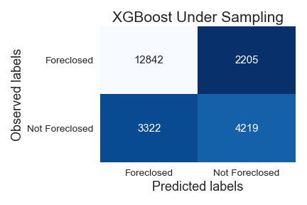
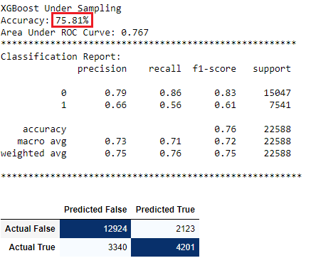
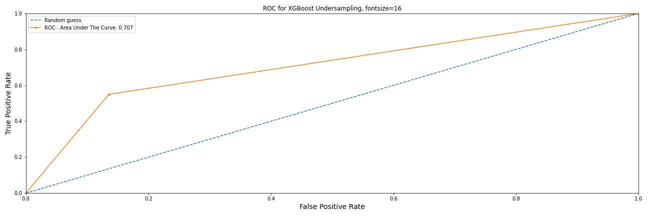
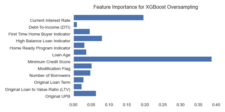
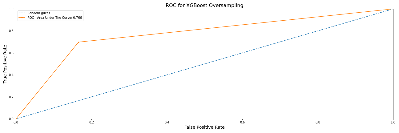
XGBoost
XGBoost Under Sampling Data
Feature Importance
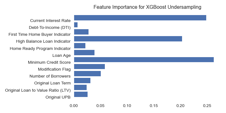
XGBoost Under Sampling Data
Feature Importance
I would like to thank Drew Jones for providing support and being an excellent listener.
Oswald Vinueza thank you for answering all my questions and providing direction when needed.
August 2nd app was uploaded to docker
August 3rd app was deployed on AWS